NumProg Summary

$\qquad\qquad\qquad\qquad\qquad \text{\it by jws}$

Overview (and Todos)

1. Floating Points, Rounding, Condition & Stability, Cancellation

2. Interpolation:

   • with polynomials
   • with splines
   • with trigonometric functions / DFT

3. Numerical Quadrature (Integrals)

   • rectangle rule
   • trapezoidal rule
   • Kepler's rule
   • ...

4. Solving Linear Systems Directly

   • Gaussian Elimination
   • LU factorization
   • Cholesky factorization
   • Pivot search

5. Ordinary Differential Equations (ODE)

   • Separation of variables
   • One-step methods:
     • Euler method
     • Heun method
     • Runge and Kutta method
   • Local & Global discretization error
   • Multistep methods:
     • Adams-Bashforth method
   • Stiffness
   • Implicit methods:
     • Implicit Euler method

6. Iterative Roots and Optima

   • Relaxation methods
     • ...
   • Minimization methods
     • ...
   • Non-linear methods
     • ...
   • Multigrid

7. Symmetric Eigenvalue Problem

8. Hardware-Aware Computing

   • Space-filling curves
   • Matrix multiplication

TODO:

• saturday 1-4
• sunday 5-8
• monday altklausuren & coding
• tuesday party

0. Error Analysis:

Exact value $x$ gets perturbed with error and becomes perturbed value $\tilde x$:
Absolute error $\delta x := \tilde x - x \implies \tilde x = x + \delta x$
Relative error $\varepsilon := \frac{\tilde x - x}{x} = \frac{\delta x}{x} \implies \tilde x = x(1 + \varepsilon)$
similarly, absolute output error = $f(\tilde x) - f(x)$ and relative output error = $\frac{f(\tilde x) - f(x)} {f(x)}$

Two equivalent ways to view perturbation of operation $a \dot + b$:
Forward analysis: exact input $a, b \rarr$ exact result $a + b \rightsquigarrow$ perturbed result $(a+b)(1+\varepsilon)$
Backward analysis: exact input $a, b \rightsquigarrow$ perturbed input $a(1+\varepsilon), b(1+\varepsilon) \rarr$ "exact" result $a(1+\varepsilon) + b(1+\varepsilon)$
$\qquad\qquad\qquad a \dot \cdot b = \underbrace{(a \cdot b) (1 + \varepsilon)}_\text{forward} = \underbrace{(a \sqrt{1+\varepsilon}) \cdot (b \sqrt{1+\varepsilon})}_\text{backward}$

Condition: sensitivity of output according to input perturbation (>1: amplification of error) inherent to the problem, not the used algorithm
$\text{abs cond} := \frac{\text{abs output error}}{\text{abs input error}}$, $\text{rel cond} := \frac{\text{rel output error}}{\text{rel input error}}$
Approximation with derivative: $cond(f, x) = |\frac{x \cdot f'(x)}{f(x)}|$
Chaining of compound problems: $cond(f(x)) := \frac{\partial f(x)}{\partial x}$

Stability: an algorithm is stable, if all perturbed inputs produce acceptable results:
An approximation $\tilde y(x)$ is acceptable if it's the exact solution to a perturbed input: $\tilde y(x) = p(\tilde x)$ (thus if the problem is ill-conditioned, $\delta y$ can be large and still be acceptable)
Stability analysis with Epsilontik: ...

Cancellation: when subtracting two very similar numbers ($1000 - 999$), even very small relative input error $\pm \frac{1}{1000}$ can lead to high relative output error ($= 2$) which causes the relative condition number to explode ($2000$), even worse for complete cancellation (exact result = 0) $\implies cond = \infin$!

1. Floating Point Numbers

Discretization of $\R$, without the disadvantages of fixed point (fixed range, overflow, too little precision at small numbers and wasted precision at big numbers, ...)

Normalized $t$-digit floating point to basis $B$ (machine number):

$\mathbb{F}_{B,t,\alpha,\beta} = \{ M \cdot B^E \mid M=0 \lor \underbrace{B^{t-1} \leq |M| < B^t}_{\Rightarrow\ t \text{ digits, no leading 0}},\ \underbrace{\alpha \leq E \leq \beta}_{\text{range for E}}, \text{ with } M, E \in \Z \}$

The mantissa $M$ and exponent $E$ are saved as integers, the basis $B$ and digits $t$ are ususally implicit.

The absolute distance between two neighboring floats is not constant:
$\qquad |98 \cdot 10^0 - 99 \cdot 10^0| = 10^0$
$\qquad |98 \cdot 10^1 - 99 \cdot 10^1| = 10^1$
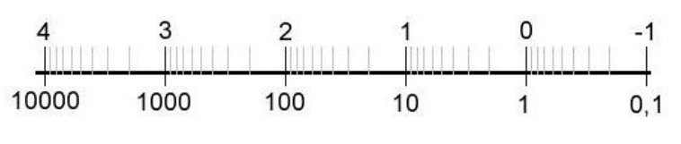
The bigger the absolute value gets, the less precision it has (logarithmic scale!)

Max relative distance = resolution $\varrho := B^{1-t} \geq \frac{1}{|M|} = \frac{(|M|+1) \cdot B^E - |M| \cdot B^E}{|M| \cdot B^E}$
Min positive float = $\sigma := B^{t-1} \cdot B^\alpha$
Max float = $\lambda := (B^t - 1) \cdot B^\beta$

Rounding function $rd(x)$ maps every $x \in \R$ to a $f \in \mathbb{F}$

• they should be surjective, idempotent and monotone
• if $x \in \mathbb{F}$, then $rd(x) = x$
• if $x \in \R \setminus \mathbb{F}$, then every $x := (M + \delta) \cdot B^E,\text{ with } \delta \in (0; 1)$ has a neighbor to left/right:
  $\quad f_l(x) := max\{ f \in \mathbb{F} \mid f \leq x \} = M \cdot B^E$
  $\quad f_r(x) := min\{ f \in \mathbb{F} \mid f \geq x \} = (M+1) \cdot B^E$
• rounding down: $rd_-(x) := f_l(x)$, rounding up: $rd_+(x) := f_r(x)$
• chop off (= towards zero): $rd_0(x) := \begin{cases} f_l(x) & \text{if } x \geq 0 \\ f_r(x) & \text{if } x \leq 0 \end{cases}$
• correct rounding (= towards closest): $rd_*(x) := \begin{cases} f_l(x) & \text{if } x < m \\ f_r(x) & \text{if } x > m \end{cases} \text{ with } m := \frac{f_l(x)+f_r(x)}{2}$
• if x is exactly in the middle, choose what to do!
• absolute rounding error: $rd(x) - x$
• relative rounding error: $\varepsilon := \frac{rd(x)-x}{x} \implies rd(x) = x \cdot (1+\varepsilon)$
• machine accuracy $\bar \varepsilon \geq |\varepsilon|$: directed rounding: $\bar \varepsilon := \varrho$, correct rounding: $\bar \varepsilon := \varrho / 2$
• the weak hypothesis (see Lec.1 P.27) only allows for backward analysis, the strong allows for both

A floating point arithmetic $\dot *$ is ideal if it's the rounded exact result: $a \dot * b= rd(a * b) = (a * b) \cdot (1 + \varepsilon(a, b))$
Most floating point operators are not associative anymore!

IEEE-Standard Floats:

• 32-bit:

  • 1 bit: sign ($0 = +, 1 = -$)
  • 8 bits: $E + 127 \implies E = 8bits - 127$, -127 and +128 reserved
  • 23 bits: $|M| = 1.[23bits]$ (normalized with leading 1)
  • rounding: correct rounding + for exact middle (0.1): round towards even number

• 64-bit;
  ...

2. Interpolation

Given $n$ support points $(x_i, y_i)$ of function $f(x)$, build an approximant $p(x)$ that goes through them: $\forall i: p(x_i) = y_i$
mesh width $h_i := x_{i+1} - x_i$

Lagrange interpolation: Only support points are given
Hermite interpolation: Each support points additionally have required derivative $y'_i$

Interpolation using polynoms:

• Simple approach: Find coefficients of general term $p(x) := \sum_{i=0}^n a_i \cdot x^i$ by solving the system of equations for each support point $(x_i, y_i)$

• Lagrange polynomial: $L_k(x) := \prod_{i:i \neq k} \frac{x-x_i}{x_k-x_i}$ with property that it equals 0 for all nodes except $x_k$, and becomes 1 at node $x_k$
  Therefore $p(x) := \sum_{i=0}^n y_i \cdot L_i(x)$ is a valid polynomial interpolant.

• Scheme of Aitken and Neville: Instead of explicitly finding the term $p(x)$, calculate the interpolated value for a concrete $x$

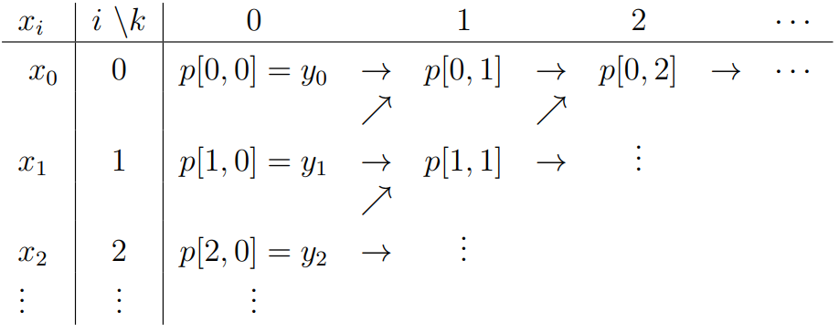
  • Define auxiliary polynomials $p_{i,k}(x)$ which are polynomials of degree $k$ and interpolate the support points in $[i; i+k]$ (thus base case $\forall i: p_{i,0}(x) = y_i$)
  • Recursive formula: $p_{i,k}(x) = \frac{x_{i+k} - x}{x_{i+k} - x_i} \cdot p_{i, k-1}(x) + \frac{x - x_i}{x_{i+k} - x_i} \cdot p_{i+1, k-1}(x)$
    
  • Then $p(x) := p_{0,n}(x)$ (if instead recursive formula is evaluated, the full term $p(x)$ can be determined)

• Newton's Interpolation Formula: Another recursive formula, but incremental, i.e. when another node $x_{n+1}$ is added, only one new summand has to be added!

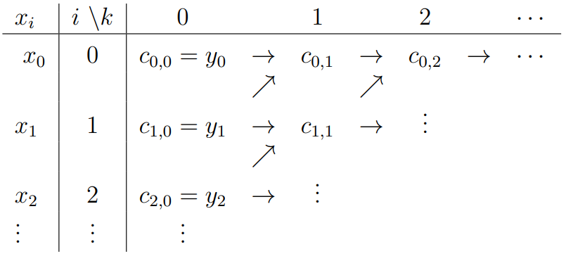
  • The divided difference of $p_{i,k}$ is the coefficient of the highest degree term $x^k$: $[x_i,...,x_{i+k}]f =: c_{i, k}$ (thus base case $\forall i: c_{i,0} = y_i$)
  • Recursive formula: $c_{i,k} = \frac{c_{i+1,k-1} - c_{i,k-1}}{x_{i+k} - x_i}$
    
  • Then $p(x) := c_{0,0} + c_{0,1} \cdot (x-x_0) + ... + c_{0,n} \cdot \prod_{i=0}^{n-1} (x-x_i)$

• Error of polynomial interpolants: For a concrete intermediate point $\bar x$, its error $|f(\bar x) - p(\bar x)|$ is in $O(h^{n+1})$ for equidistant mesh width $h$:
  $\Rightarrow$ lower $h$ and higher $n$ should decrease error in theory (but due to Runge effect, not in practice!)

  • Equidistant nodes not optimal! (Chebychev nodes to add more nodes at the edges is optimal)

• Condition of polynomial interpolants: Sensitivity of error in $p(x)$ regarding error in $y_i$

  • derivative of $y$ regarding $y_i$ is $L_i(x)$, but small errors in central supporting values are dramatically increased at the borders of the interpolation interval!
  • for large n (7+ or 8+), extremely ill-conditioned for equidistant nodes

Interpolation using Polynomial Splines: Glue together pieces of polynomials of lower degree to avoid expensive computation and the Runge effect

• Spline $s: [a; b] \rarr \R$ of order $m$ / degree $m-1$:
• $s(x) = p_i(x)$ on $[x_i; x_{i+1}]$, $n$ pieces of polynomials between each knots ($n+1$ knots)
• Locally: Between two knots, polynomial of degree $m-1$ ($p_i \in \mathbb{P}_{m-1}$)
• Globally: $s$ is $m-2$ times continuously differentiable ($s \in C^{m-2}([a;b])$)
  $m=1$: step function (piecewise continuous, not really a spline)
  $m=2$: linear interpolation (knots are connected, not really spline either)
  $m=3$: quadratic spline (knots have no sharp bends)
  $m=4$: cubic spline (continuous 1st & 2nd derivatives)
• $n+m-1$ degrees of freedom (of which $n+1$ knot contraints are given)

Cubic Splines ($m=4$): Each piece is a cubic polynomial with parameters $y_i$, $y_{i+1}$, $y_i'$, $y_{i+1}'$:
$s(x) := p_i(t)$ where $t$ linearly connects from $(x_i; 0)$ to $(x_{i+1}; 1)$: $t := \frac{x-x_i}{x_{i+1}-x_i}$
then $p_i(t) := y_i \cdot \alpha_1(t) + y_{i+1} \cdot \alpha_2(t) + (x_{i+1} - x_i) \cdot (y_i' \cdot \alpha_3(t) + y_{i+1}' \cdot \alpha_4(t))$ (see Lec.2 P.31 for $\alpha_i$ def.)

To determine the $y_i'$s such that the 2nd derivatives at the knots are continuous, solve $p_{i-1}''(1) = p_i''(0)$ for all $y_i$s (tridiagonal system of linear equations of dim $n-1$)
The remaining 2 degrees of freedom $y_0', y_n'$ are boundary conditions, either given directly, set by given 2nd derivatives, or such that it's periodic ($y_0' = y_n'$ and $s''(x_0) = s''(x_n)$)

Cost: Tridiagonal system of equations can be solved in $O(n)$ as opposed to $O(n^3)$ for a full system, or the $O(n^2)$ for Aitken and Neville / Newton

Error: Since we're using cubic polynomials, $|f(x)-s(x)| = O(h^4)$

Trigonometric Interpolation: Given $n$ nodes on the unit circle $z_j := e^{2\pi i j / n}$ (equally spaced on the circle edge) and their corresponding values $v_j$, find the interpolant $p(z)$ where $z := e^{2\pi i t}, t \in [0; 1]$ such that $\forall j: p(z_j) = v_j$
General representation as a linear combination of exponential functions:
$p(z) := \sum_{k=0}^{n-1} c_k z^k = \sum_{k=0}^{n-1} c_k e^{2 \pi i k t}$ (can be separated into $cos$ and $sin$)
Find the coefficients $c_k \implies$ Discrete Fourier Transform:

• for $\omega := e^{2 \pi i / n}, M = (\omega^{jk})$, solve $\vec v = IDFT(\vec c) := M \cdot \vec c\ {}$ or $\ \vec c = DFT(\vec v) := \frac{1}{n} \cdot \overline M \cdot \vec v$, which takes $O(n^2)$
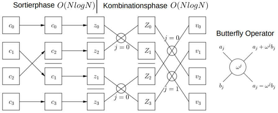
• the Fast Fourier Transform can calculate $v = IDFT(c)$ in $O(n\ log\ n)$ through recursion, halving $n = 2m$, $j \in [0; m-1]$:
  $v_j = IDFT(c_0, c_2, ...) + \omega^j \cdot IDFT(c_1, c_3, ...)$
  $v_{j+m} = \underbrace{IDFT(c_0, c_2, ...)}_{\text{even coefficients}} - \omega^j \cdot \underbrace{IDFT(c_1, c_3, ...)}_{\text{odd coefficients}}$
• Easier to visualize:
  

Cosine Transform?: ...

3. Numerical Quadrature

Given function $f: [a; b] \rarr \R$, calculate definite integral $I(f) := \int_a^b f(x) dx$ using approximant rules of quadratures, which are weighted sums of samples $(x_i, y_i)$:
$I(f) \approx Q(f) := \sum_{i=0}^n g_i \cdot y_i$ with weights $g_i$ (thus: find appropriate weights!)
We can use polynomial interpolation $p(x)$ of $f(x)$ to find the weights:
$Q(f) := \int_a^b p(x)dx = \int_a^b \sum y_i L_i(x) dx \implies g_i := \int_a^b L_i(x)dx$
$\qquad$($L_i$ only depends on $x_i$; weights can be pre-calculated!)
$\qquad$(since $\sum_i L_i(x) = 1 \implies \sum_i g_i = b - a$)

Condition of quadrature: For input error $|\delta y_i| \leq \varepsilon$, its output error $\delta Q(f)$ has the upper bound $|\delta Q(f)| \leq \varepsilon \cdot \sum_i |g_i|$, which depends on the weights:
$\forall i: g_i \geq 0 \implies \sum_i |g_i| = b - a \implies$ well-conditioned $O(\varepsilon)$!
$\exists i: g_i < 0 \implies \sum_i |g_i| > b- a \implies$ ill-conditioned! (occurs at big $n$)

Simple rules of quadrature calculate the result of the entire $[a;b]$ at once ($H := b-a$):

• The rectangle rule $Q_R(f) := H \cdot f(\frac{a+b}{2}) = H \cdot y_0$ takes one sample point in the middle $x_0 := (a+b)/2$ (exact integral of constant interpolant)
  Its remainder $R_R(f) = -H^3 \cdot \frac{f^{(2)}(\xi)}{24}$ for intermediate point $\xi \in (a; b)$; thus $Q_R$ is exact for $f \in \mathbb{P}_0$ or $\mathbb{P}_1$ (order 3; degree of accuracy = 1)
• The trapezoidal rule $Q_T(f) := H \cdot \frac{f(a) + f(b)}{2} = H \cdot \frac{y_0 +y_1}{2}$ takes two sample points $x_0 := a$ and $x_1 := b$ (exact integral of linear interpolant)
  Its remainder $R_T(f) = H^3 \cdot \frac{f^{(2)}(\xi)}{12}$ again exact for $f \in \mathbb{P}_0$ or $\mathbb{P}_1$ (order 3; accuracy 1)
• The Kepler's rule $Q_F(f) := H \cdot \frac{f(a) + 4 f((a+b)/2) + f(b)}{6} = H \cdot \frac{y_0 + 4y_1 + y_2}{6}$ takes three sample points $x_0 := a$, $x_1 := (a+b)/2$, $x_2 := b$ (exact integral of quadratic interpolant)
  remainder $R_F(f) = H^5 \cdot \frac{f^{(4)}(\xi)}{2880}$; thus order 5 and accuracy 3
• The Newton-Cotes formula generalizes this increasing sample points and order: $Q_{NC}(f) := I(p_n)$ where $p_n$ polynomial interpolant of degree $n$ to the $n+1$ equidistant nodes $x_0 := a, ..., x_i := a + H \cdot i/n, ..., x_n := b$
  Thus with growing $n$, the order and accuracy increases. But for $n = 8$ and $n \geq 10$, negative weights occur; very ill-conditioned!
• The Clenshaw-Curtis rules uses non-uniformly distributed nodes (Chebychev nodes: x component of uniformly subdivided angles on a semicircle) to completely avoid negative weights: $x_i := a + H \cdot (1- cos(i \pi / n)) / 2$
  Thus can be used for large $n$ without being ill-conditioned (but composite rules are more practical)

Composite rules of quadrature split the integration domain $[a;b]$ into $n$ subdomains of length $h := (b-a) / n$, applies simple rules and sums up, just like splines!

• The trapezoidal sum applies the trapezoidal rule between each nodes: $Q_{TS}(f; h) := h \cdot (\frac{y_0}{2} + y_1 + ... + \frac{y_n}{2})$ (therefore weights $g_0 := h/2 =: g_n, \text{ otherwise } g_i := h$), integral of linear splines!)
  Its remainder $R_{TS}(f; h) = h^2 \cdot H \cdot \frac{f^{(2)}(\xi)}{12}$ (order decreased by 1 to 2; accuracy still 1), $n$ can grow without condition problem
• The Simpson sum applies the Kepler's rule to each node pairs (without overlap): $Q_{SS}(f;h) := \frac{h}{3} \cdot (y_0 + 4y_1 + 2y_2+ 4y_3 + ... + y_n)$ (alternates between 4 $\lrarr$ 2 and 1 on each ends)
  remainder $R_{SS}(f;h) = h^4 \cdot H \cdot \frac{f^{(4)}(\xi)}{180}$ (order decreased by 1 to 4; accuracy still 3), $n$ can also grow without condition problem

Extrapolation: Express the quadrature as exact value + error (Euler-Maclaurin sum formula, if $f \in C^{2m}$):
$Q_{TS}(f; h) = \underbrace{I(f)}_\text{exact} + \underbrace{\tau_1 h^2 + ... + \tau_{m-1} h^{2m-2} + \tau_m(h) \cdot h^{2m}}_\text{error} =: T(h)$

• You could linearly combine different $h_i$ values to reduce the error (first eliminate the unknown factor $\tau_1$, then $\tau_2$, etc...)
• Alternative perception of the Romberg quadrature: $h \to 0 \implies T(h) \to I(f)$ exact integral, therefore interpolate $T(h)$ with $p \in \mathbb{P}_{m-1}$ in the nodes $(h_i^2, T(h_i)), i \in [1;m]$ and use $p(0)$ as approximation of $I(f)$ (calculate $p(0)$ with Neville's scheme)
• The error $|I(f) - p(0)|$ is in $O(h_1^2 \cdot h_2^2 \cdot ... \cdot h_m^2)$, which is significantly better than the trapezoidal rule (but $f$ must be $2m$-times continuously differentiable!)